In a previous post, I introduced Movie Explorer, a simple movie recommender implemented in SQL. This specific type of recommendation is known as Example-Critiquing. Users can search for a movie (the example) and then see similar results based on modifications to that movie (the critiques). This allows users to express something akin to show me movies like X but with more Y and less Z.
In this post, I will describe how I implemented the recommendation logic and the challenges I faced during development.
TL;DR
- Similarity is calculated using cosine similarity between vectors of tags.
- Critiques are applied to an example by modifying the tag vector.
- Being able to explain similarity scores is crucial for improving the results.
- It is important to know the dataset in detail.
- Subject matter expertise is critical.
Defining Movie Similarity
It is worth reflecting on what it means for movies to be similar. There are many different ways in which movies could be considered similar: language, genre, cast and crew, setting (both location and period), country of production etc etc. Sometimes movies might be considered similar if they share a certain sensibility but differ in most other regards.
If you were to ask a movie enthusiast to recommend similar movies you might find that they would choose to place more or less emphasis on certain aspects depending on the movie in question and the person asking. In this regard, similarity isn’t a stable and unchanging quality.
Whenever undertaking any kind of recommendation project, I think it is valuable to answer these kinds of questions before rushing to specific approaches based on convenience.
For Movie Explorer I decided to use tags as the basis for similarity. Movies that have very similar tags and tag scores are considered to be similar.
Tags and Tag Scores
I’ll be using the GroupLens Tag Genome 2021 Dataset:
10.5 million computed tag-movie relevance scores from a pool of 1,084 tags applied to 9,734 movies. Released 12/2021.
The dataset is based on user-submitted tags on MovieLens. Each tag has a relevance score between 0 (does not apply) and 1 (absolutely applies). For example, Lost In Translation has a score of 0.85 for the tag melancholic, which means that is quite melancholic but could be more so.
Tags created by users present two main challenges:
- Users often use different phrases or spellings for the same tag.
- Tags are not consistently applied to all movies.
The Tag Genome dataset applies an algorithm to present a consistent set of tags for a subset of movies. This fact will come back to haunt me.
Calculating Cosine Similarity
Now that we have some tags and tag scores for our set of movies we can define similarity using Cosine Similarity.
We take the set of tags and their scores to constitute a vector for each movie and then we calculate the cosine of the angle between these vectors. Since our tag scores are never negative our results will always lie in the interval [0,1], where 0 is a movie pair with no similarities at all (an orthogonal vector) and 1 is a movie pair with perfect similarity (a proportional vector).
The cosine can be defined in terms of the dot product of vectors, divided by the product of their magnitudes.
\(\cos \theta = {\textbf{A} \cdot \textbf{B} \over \Vert\textbf{A}\Vert \Vert\textbf{B}\Vert} \)
We can simplify this by converting our vectors to unit vectors, in which case the denominator is always 1.
\(\cos \theta = \textbf{A} \cdot \textbf{B}\)
By definition, this is equivalent to:
\(\cos \theta = \sum_{i=1}^n {A_i}{B_i}\)
Calculating a dot product in SQL can be expressed very easily. The query below assumes the existence of a table called movie_tags_unit_score in which each row has the following:
- Movie identifier (
item_id) - A label identifying a tag (
tag) - Tag unit score: this is the score for the tag in the unit vector representation of the tag vector for the movie. (
unit_score) - It will prove useful to keep the raw tag score on hand too as this will allow us to fine-tune the results by redefining the values for the tags for a specific movie before computing an updated unit vector representation.
WITH similarities AS (
    SELECT
        lhs.item_id as reference_movie_id,
        rhs.item_id as comparison_movie_id,
        SUM(lhs.unit_score * rhs.unit_score) as similarity_score
    FROM `movielens.movie_tags_unit_score` lhs
    INNER JOIN `movielens.movie_tags_unit_score` rhs ON lhs.tag = rhs.tag
    WHERE lhs.item_id = @lhs_item_id
        AND lhs.item_id <> rhs.item_id
    GROUP BY 1, 2
),
ranked_similarities AS (
    SELECT
        similarities.comparison_movie_id as movie_id,
        similarities.reference_movie_id,
        similarities.similarity_score,
        RANK() OVER (PARTITION BY similarities.reference_movie_id
                     ORDER BY similarities.similarity_score DESC) as similarity_rank
    FROM similarities
)
SELECT
  *
FROM ranked_similarities
WHERE similarity_rank <= @results_per_movie
One of the benefits of this approach (besides its simplicity) is that it will allow us to easily inspect the components of our computed similarity scores and understand why specific pairs of movies are very similar or dissimilar.
Applying Critiques To The Example Movie
The user can apply critiques to the example movie by selecting tags to be boosted or penalised in the calculation. We modify the tag vector for the example movie by increasing or decreasing the scores for the specified tags and then use that vector as the new example for the similarity query.
Evaluating Results
One of the many challenges with recommender systems is that there is no baseline for truth. We cannot compare our results to an expected set of results.
Below we consider the results for the top five movies most similar to Lost In Translation (2003).
Movies similar to Lost In Translation (2003)
| Similarity Rank | Title | Similarity Score |
|---|---|---|
| 1 | Broken Flowers (2005) | 0.894436 |
| 2 | In the Mood For Love (Fa yeung nin wa) (2000) | 0.884621 |
| 3 | Punch-Drunk Love (2002) | 0.882073 |
| 4 | Magnolia (1999) | 0.874004 |
| 5 | Sideways (2004) | 0.873383 |
Broken Flowers (2005) and In The Mood For Love (2000) are both fairly good results. Magnolia (1999) is a very poor result for the top five. There is very little that is similar between the movies.
We can now take advantage of our ability to view the components of the similarity score at the tag level to see where this result goes off the rails.
Examining Similarity Between Magnolia And Lost In Translation
Let us consider the top twenty tags that contributed to the similarity score for Lost In Translation and Magnolia.
| Tag | Lost In Translation Score | Magnolia Score | Cumulative Percentage of Similarity |
|---|---|---|---|
| midlife crisis | 1.007973 | 1.002816 | 0.992071 |
| original | 0.993752 | 1.014088 | 1.981140 |
| relationships | 0.990892 | 1.000181 | 2.953837 |
| golden palm | 0.969133 | 1.017708 | 3.921846 |
| beautifully filmed | 0.983539 | 0.950735 | 4.839594 |
| visually appealing | 0.976246 | 0.953849 | 5.753521 |
| very interesting | 0.950248 | 0.903615 | 6.596259 |
| loneliness | 0.984463 | 0.846032 | 7.413704 |
| good soundtrack | 0.853977 | 0.969064 | 8.225920 |
| good music | 0.851935 | 0.971075 | 9.037875 |
| movielens top pick | 0.883924 | 0.933557 | 9.847769 |
| great soundtrack | 0.826765 | 0.946215 | 10.615562 |
| oscar (best directing) | 0.763731 | 0.997399 | 11.363184 |
| criterion | 0.838667 | 0.894395 | 12.099377 |
| life & death | 0.867713 | 0.857749 | 12.829858 |
| creativity | 0.808601 | 0.913394 | 13.554737 |
| great cinematography | 0.892945 | 0.820487 | 14.273804 |
| character study | 0.882385 | 0.829649 | 14.992301 |
| dialogue | 0.922033 | 0.783600 | 15.701412 |
| art | 0.906294 | 0.795164 | 16.408703 |
Analysing the Similarity Components
It is worth pausing to consider the individual tags and how their meaning may contribute to (or detract from) our current project of determining movie similarity. Not all tags are equally useful for the purpose of determining similarity.
Three main challenges arise from the tags and values in terms of our current approach:
- Tag quality and relevance.
- Tags with low scores account for too much similarity.
- Individual tags contribute too little to the overall score for effective tuning.
Tag Quality and Relevance
A close inspection of the tag data reveals many problems. Many tags are irrelevant or redundant. In some instances, the tag might be relevant but the computed score for some movies is inaccurate.
Redundant Tags
How is indie different from independent film? Is great cinematography really that different from beautifully filmed? And what about good cinematography or perhaps just cinematography?
Magnolia gets a few percent of its similarity from good soundtrack, great soundtrack and good music.
Including redundant tags does little to increase the information in the dataset but detracts from determining overall similarity as it effectively boosts these concepts.
Tags About External Factors
Many tags are related to awards such as the Palme d’Or (the tag golden palm) or the Oscars. Other tags are about being in the Criterion Collection or being a Movielens Top Pick. These tell us little about the movies themselves.
Tags About Cast/Film Series
Many tags refer to a director or actor. In some cases these contain surprising values. I have seen Francis Ford Coppola movies that score high on the tag martin scorsese. Other tags refer to film series, e.g. batman, 007, harry potter.
While it could be argued that these sorts of tags are useful in terms of determining similarity I think that this is a poor basis for using similarity for discovery.
Low Scoring Tags Account For Too Much Similarity
Fifteen percent of the similarity between Broken Flowers and Lost In Translation comes from tags where both movies score quite low such as grindhouse, irish accent and gratuitous violence.
Having a tag score below a certain threshold tells us close to nothing about a movie but contributes too much to the overall similarity score.
Individual Tag Contribution Is Too Low For Movie Tuner
If you were to use our proposed approach of querying for movies similar to Lost In Translation but with less midlife crisis the results would be largely the same, even though it is the largest component for multiple of the top results. Broken Flowers would still be the top result.
The individual tags that we might want to increase or decrease in our queries contribute too little to the overall result to make a significant difference unless we modify a large number of them.
Pruning The Tags
One approach to improving our results would be to apply some careful pruning to the existing tags for all movies.
Reducing Redundant Tags
Identifying redundant tags and selecting only one for each group will improve the information content for each movie.
Potentially redundant tags can be identified by finding the correlation between tag scores at the movie level. Some tags may be correlated but distinct, such as horror and gore. Other tags, such as vampire and vampires, are effectively synonyms.
Some human judgment is required in determining what to keep and what to drop.
SELECT
  lhs_tags.tag as lhs_tag,
  rhs_tags.tag as rhs_tag,
  CORR(lhs_tags.score, rhs_tags.score) as correlation
FROM movielens.movie_tags lhs_tags
INNER JOIN movielens.movie_tags rhs_tags ON rhs_tags.item_id = lhs_tags.item_id
WHERE lhs_tags.tag <> rhs_tags.tag
GROUP BY lhs_tag, rhs_tag
ORDER BY correlation DESC
LIMIT 20
| lhs_tag | rhs_tag | correlation | |
|---|---|---|---|
| 0 | 007 | 007 (series) | 0.956590 |
| 1 | 007 (series) | 007 | 0.956590 |
| 2 | vampire | vampires | 0.955385 |
| 3 | vampires | vampire | 0.955385 |
| 4 | superhero | super hero | 0.952495 |
| 5 | super hero | superhero | 0.952495 |
| 6 | harry potter | emma watson | 0.940004 |
| 7 | emma watson | harry potter | 0.940004 |
| 8 | james bond | 007 | 0.930896 |
| 9 | 007 | james bond | 0.930896 |
| 10 | 007 (series) | james bond | 0.929199 |
| 11 | james bond | 007 (series) | 0.929199 |
| 12 | alien | aliens | 0.919349 |
| 13 | aliens | alien | 0.919349 |
| 14 | superhero | super-hero | 0.909674 |
| 15 | super-hero | superhero | 0.909674 |
| 16 | oscar (best supporting actor) | oscar (best directing) | 0.908535 |
| 17 | oscar (best directing) | oscar (best supporting actor) | 0.908535 |
| 18 | sci-fi | scifi | 0.900247 |
| 19 | scifi | sci-fi | 0.900247 |
Remove Irrelevant Tags
Many tags have very little relevance to our task, such as imdb top 250 and harry potter. Removing these tags increases the contribution of more meaningful tags to the similarity score.
Reduce Tags At The Movie Level
Pruning tags with lower scores can be done by either applying a value threshold or by simply selecting the top N tags for each movie and dropping the rest.
Below we consider the distribution of tag scores for 30th, 50th and 100th rank for each movie.
%%bigquery tag_ranks
WITH ranked_tags AS (
    SELECT
        item_id,
        score,
        RANK() OVER (PARTITION BY item_id ORDER BY score DESC) as tag_rank
    FROM movielens.movie_tags
)
SELECT
    *
FROM ranked_tags
WHERE tag_rank IN (30, 40, 50, 100)
from plotnine import ggplot, geom_histogram, aes, stat_smooth, facet_wrap

(ggplot(tag_ranks) +
    aes(x="score",
        fill="factor(tag_rank)") +
    geom_histogram(alpha=0.5, binwidth=0.02) +
    facet_wrap("~tag_rank"))
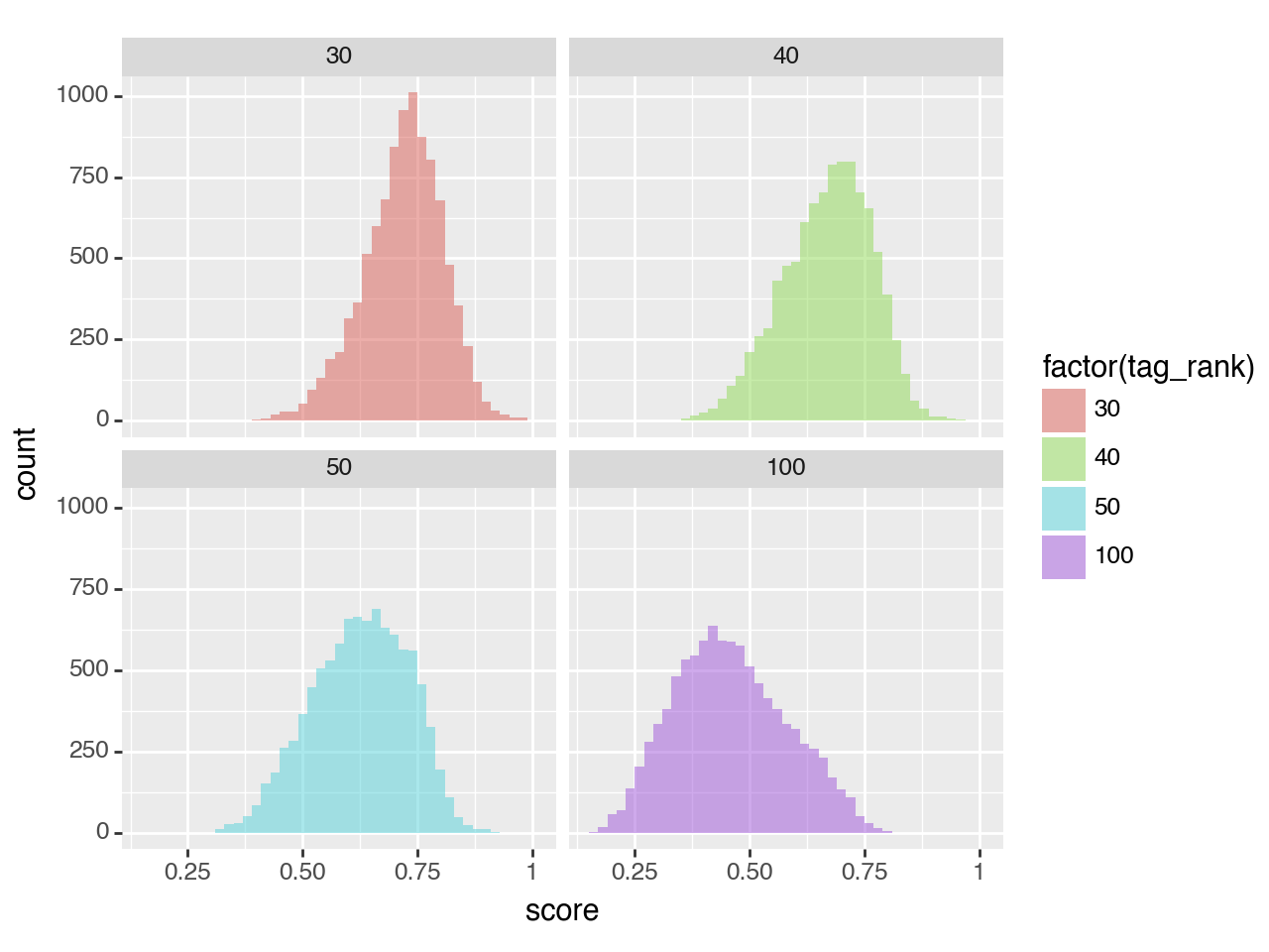
I elected to keep the top 40 tags for each movie. An additional benefit of this approach is that it radically reduces the number of rows that need to be aggregated for each similarity calculation.
Refined Similarity Results
Having applied the above improvements, let us revisit the results for Lost in Translation.
| Similarity Rank | Title | Similarity Score |
|---|---|---|
| 1 | In the Mood For Love (Fa yeung nin wa) (2000) | 0.643143 |
| 2 | Fallen Angels (Duo luo tian shi) (1995) | 0.581406 |
| 3 | Yi Yi (2000) | 0.580614 |
| 4 | Vertical Ray of the Sun, The (Mua he chieu tha... | 0.580127 |
| 5 | Junebug (2005) | 0.567591 |
Magnolia is no longer a top match and the other recommendations are moving in the right direction. The similarity scores are much lower (previously these were high 0.80s) but this decrease is a good thing because we were aiming to reduce semantic redundancy.
These results are more interesting to me because I want to discover movies that are new to me or that I was aware of but might not have otherwise considered.
Implementation
My initial plan was to do everything using Google Cloud Platform. One of my main requirements was a solution that didn’t cost anything if it wasn’t being used. Enter Google Cloud Functions, BigQuery, Pubsub, Firestore, etc etc. I started down this route and found that the overhead of using and configuring these tools was getting in the way of actually iterating on the results of the algorithm.
With my much more compact dataset in hand, I decided to see how far I could get with Duck DB and Streamlit. This combination of tools worked admirably well for what I wanted to achieve. Calculating similarity is fast enough that nothing needs to be cached, which means that the datastore can be read-only. Streamlit is a great tool and they offer free hosting.
These two tools allowed me to iterate very quickly.